[RNH post #14] Final Project Report

Hi all! 

The GSoC coding period is now over!

Having participated on the GSoC was an amazing experience. In general, all objectives of my project were accomplished. Now, the scientific and wider imaging processing community can have access to the first open source DKI processing modules. As the results of this project showed (see for example my post #10 and post #11), this modules can be used to analyse data of large world wide collaborative projects such as the Human Connectome Project (HCP). Moreover, I had a great time working with members of my mentoring organization - I learned a lot with them and I will definitely continue contributing with Dipy in the following years.

Below you can find my final project report.

Project summary

In sum, this project was organized in 4 main phases: 1) finishing the work done on functions to simulate signal from the DKI model; 2) implementing methods for estimating the diffusion kurtosis tensor and derived measures; 3) adding a procedure to estimate biophysical parameters from DKI; and 4) developing techniques to estimate fiber directions from real DKI data. The details of the work done on each phase is described below:

DKI based simulations

In this part of the project, I implemented the DKI simulates that were important to test the performance of all functions created on the other steps of the project. Part of this work was done before the GSoC coding period and its finalization was reported in the midd-term summary. Just to highlight the relevance of these simulations, during the GSoC coding period, 19 nose tests functions  were created in which 13 were based on DKI based simulates. Moreover, DKI simulations were also useful for selecting, optimizing and debugging DKI methods (see for example post #9 and post #13).

DKI reconstruction modules

As I proposed in my initial project plan, having a final version of the DKI fitting modules and estimation of diffusion kurtosis statistics was the main goal to achieve for the midd-term evaluation. Since these modules provide the base for the work of the other parts of the project, I decided to dedicate some more time of the second half part of the GSoC coding period to improve the diffusion kurtosis statistics functions. These improvements are summarized in the following points:

• The analytical solutions of the mean and radial kurtosis were validated using two numerical methods (post #9).
• The performance of the functions were improved so that all standard kurtosis statistics can be computed within 1 min (post #10)
• I also explored some Dipy's pre-processing steps that dramatically improved the quality of the DKI reconstructions (post #11 and post #12).
• I added some nosetests to insure that all code lines of DKI reconstruction modules were covered by nosetest units. From this, I detected some problems with singularities on the function computing the mean kurtosis, which were solved as reported in post #13).
• The sample usage script of these modules was adapted according to a new DKI dataset which was required with similar parameters to the HCP.

Below we show the kurtosis statistics images obtained from the HCP-like data using the DKI reconstruction modules before (upper panels of Figure 1) and after (lower panels of Figure 1) the improvements done on the second half part of the GSoC term.

Figure 1 - Diffusion Kurtosis statistics of the HCP-like data obtained from the implemented DKI reconstructions before (upper panels) and after (lower panels) the optimization done on the second half part of the GSoC coding period. Optimized functions seem to correct the artefacts present on the white matter regions as from the splenium of the corpus callosum.

The final version of the DKI modules can be found in the following pull request.

DKI based biological measures

Given the extra work done on the previous step, the implementation of the DKI biological measures was rescheduled to the last couple of weeks of the GSoC period. These measures were obtained from the DKI based model proposed by Fieremans et al., (2011), which allows the estimation of concrete biophysical parameters from brain regions of well aligned fibers. Until the end of the coding period, great advances were done on this module. For example, Figure 2 shows the estimated values of axonal water fraction (the proportion of water presented inside the fibers) for voxels containing well-aligned fibers of the splenium and genu of the corpus callosum obtained from the current version of this DKI biophysical model.

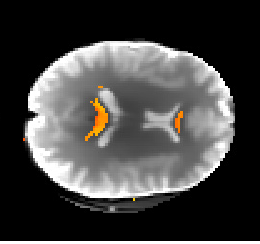
Figure 2 - Axonal water fraction values of the splenium and genu of the corpus callosum (red-yellow colormap values) plotted over the first b-value=0 of the HCP-like diffusion-weighted dataset.

Unfortunately, since the final version of these functions depends on the other pull requests that are currently being revised, the work done on the implementation of the biophysical models was not finalized, and thus it will not be submitted as part of the GSoC code sample. However, I intend to finalize soon these codes after the GSoC. If you are interested on looking to the final version of the biophysical metric estimations, keep tuned to the updates done at the DKI reconstructions pull request. 

DKI based fiber direction estimation methods 

As planed on the project proposal, in the second half part of the GSoC coding period, I developed a procedure to predict the fiber direction estimates from DKI. This was done by first estimating an orientation distribution function (ODF) which gives the probability that a fiber direction is aligned to a specific spatial direction (post #9). From the ODF, fiber directions can be estimated by finding the maxima values of the ODF (post #10). On the last couple of weeks, I accomplished a final version of this procedure by writing its sample of usage script, where real brain data ODF and fiber directions are estimated. Visualizations of these estimates are shown in Figure 3 and 4.

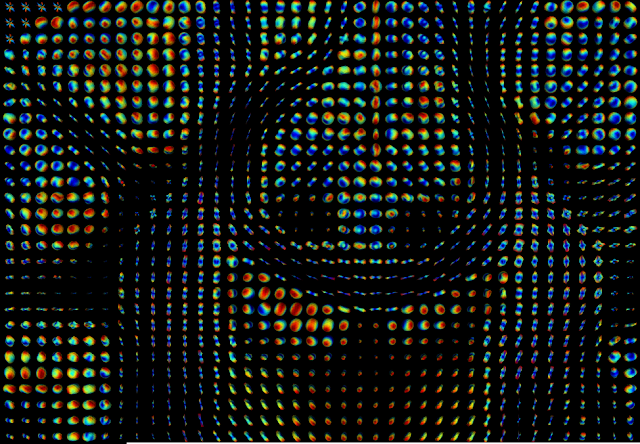
Figure 3 - DKI based orientation distribution function (ODF) computed for voxels of portion of the HCP-like data.

Figure 4 - Fiber directions computed by detecting the directions of maxima ODF. The multiple direction estimates from some voxels show that DKI is able to resolve crossing fibers.

The final version of the modules containing the function to estimate fiber directions from DKI can be found in the following pull request.

Skills gained on GSoC

• With the supervision of the members of my mentoring organization, I dramatically improve my programming skills.
• I learned all required steps to work on collaborative projects such as Dipy. Particularly, I learned how to share, update and comment my work using Github's development framework.
• I learned how to use ipython notebook to create sample script examples, and using ipython profiling techniques to check and improve function performance.
• Now I know how to use testing units, as the nosetest units, which allows me to automatically check bugs on the functions that I am implementing.
• I also learn how to improve functions using cython.
• Finally, I got familiarized with Dipy's structure and how to use their function. This is a useful knowledge for my personal future research.

[RNH post #13] Start wrapping up - Test singularities of kurtosis statistics.

As we are reaching the end of the GSoC coding period, I am starting to wrap up the code that I developed this summer.

When reviewing the code implementing the kurtosis standard statistics, I detected some problems on the performance of the analytical solution of the mean kurtosis function.

In this post, I am reporting how I overcome these issues! This post is extremely relevant for whom is interested in knowing the full details of the implementation of kurtosis standard measures.

Problematic performance near to function singularities

As I mention in previous posts, the function to compute the mean kurtosis was implemented according to an analytical solution proposed by Tabesh et al., 2011. The mathematical formulas of this analytical solution have some singularities, particularly for cases that the diffusion tensor has equal eigenvalues.

To illustrate theses singularities, I am plotting below the diffusion and kurtosis tensors of crossing fiber simulates with different intersection angles. Simulates were preformed based on the modules implemented during the GSoC coding period.

Figure 1 - Diffusion tensor (upper panels) and kurtosis tensors (lower panels) for crossing fibers intersecting at different angles (the ground truth fiber direction are shown in red).

The values of the eigenvalues of the diffusion tensor as function of the intersection angle are shown below.

Figure 2 - Diffusion eigenvalues as function of crossing fibers intersection angle. First eigenvalues is plotted in red while the second and third are plotted in green and blue.

From the figure above, we can detect two problematic cases for the MK analytical solution:

1. When intersection angle is zero (i.e. when the two fibers are aligned), the second diffusion eigenvalue is equal to the third eigenvalue.
2. When the intersection angle is 90 degrees, the first diffusion eigenvalue is equal to the second eigenvalue.

Based on the work done by Tabesh et al., 2011, these MK estimation singularities can be mathematically revolved by detecting the problematic cases and using specific formulas for each detected situation. In the previous version of my codes, I was detecting the cases that two or three eigenvalues were equal by analysis if their differences were three orders of magnitude larger than system's epslon. For example, to automatically check if the first eigenvalue equals the second eigenvalue, the following lines of code were used:

import numpy as np
er = np.finfo(L1.ravel()[0]).eps * 1e3
cond1 = (abs(L1 - L2) < er)

Although, my testing modules were showing that this procedure was successfully solving the singularities for eigenvalue differences three orders of magnitude smaller than the system's epslon, when plotting MK as function of the intersection angle, some unexpected underestimated were present on the regions near to the singularities (see the figures below).

Figure 3 - MK values as function of the crossing angle. The blue line shows the MK values estimated from the analytical solution while the red line show the MK values estimated from a numerical method described in previous posts.

Figure 4 - MK values as function of the crossing angle (range between 85 and 90 degrees). The blue line shows the MK values estimated from the analytical solution while the red line show the MK values estimated from a numerical method described in previous posts. This figure was produced for a better visualization of the underestimations still present near to the crossing angle of 90 degrees.

After some analysis, I noticed that MK underestimations were still present if eigenvalues were not 2% different to each other. Given this, I was able to solve this underestimation by adjusting the criteria of eigenvalue comparison. As example, to compare the first eigenvalue with the second, the following lines of code are now used:

er = 2.5e-2  # difference (in %) between two eigenvalues to be considered as different
cond1 = (abs((L1 - L2) / L1) > er)

Below, I am showing the new MK estimates as function of the crossing angle, where all underestimations seem to be corrected. Moreover, discontinuities on the limits between the problematic and the non-problematic eigenvalue regime are relatively small. The most significant differences are now between different MK estimation methods (for details on the difference between these methods revisit post #9).

Figure 5 - Corrected MK values as function of the crossing angle. The blue line shows the MK values estimated from the analytical solution while the red line show the MK values estimated from the numerical method described in previous posts.

[RNH post #12] Attempt to further improve the diffusion standard statistics

The denoising strategy that I used to improve the diffusion standard statistics (see my last post), required the estimation of the noise standard deviation (sigma). As a first approach, I used a simple sigma estimation procedure that was specifically developed for T1-weighted images. Thus, this might not be the most adequate approach for diffusion-weighted images.

Particularly, I noticed that sigma estimates had a dependency on the b-values (smaller b-values were related to higher sigma). Example of computed sigma for given b-values are shown bellow:

• b-value = 0 => sigma around 810
• b-value = 200 => sigma around 510
• b-value = 400 => sigma around 390
• b-value = 1000 => sigma around 268
• b-value = 2000 => sigma around 175

Comparing the original diffusion-weighted images with the denoised versions, I notice that, for the smaller b-values, some image texture was present when computing the difference between original and denoised version of the image. This suggests that sigma values for smaller b-values are overestimated.

Figure 1. - Diffusion-weighted image with b-values set to 0. Left panel shows the image before being denoised while the middle panel shows the denoised image. The difference between both images is shown in left. Some image structure can be identified on the image difference, which suggest that important information is being removed on the denoising process.

Figure 2. - Diffusion-weighted image with b-values set to 2000. Left panels show the image before being denoised while the middle panels shows the denoised image. The difference between both images is shown in left. Brain structure is not significantly identified on the image difference.

Piesno

Given the issue mentioned above, I tried to replace the noise estimation procedure with a technique specifically developed for diffusion-weighted images - a technique called piesno.
This technique can be imported and used from dipy using the follow commands:

from dipy.denoise.noise_estimate import piesno
sigma, background_mask = piesno(data, N=4, return_mask=True)

The noise standard  given by piesno for all axial images was around 156. As expected this values is smaller than the previous sigma estimates suggesting that these were indeed overestimated. 

Despite this value seems to be the most accurate estimate for the denoising procedure, I noticed that only a small amount of background voxels, used to compute sigma, was automatically detected by piesno. 

Figure 3 - Background voxels detected by piesno. These voxels were the ones used to estimate the noise standard deviation.

Computing again the difference between the original and denoised version of the data. I also notice that the denoising procedure preformance was still dependent on the b-value. In particularly, for a b-value=0 the procedure seems only to denoise the middle of the image. Since sigma was maintained constant, this dependency with the b-value seem to be caused by the denoising algorithm itself.

Figure 4. - Diffusion-weighted image with b-values set to 0. Left panels shows the image before being denoised while the middle panels shows the denoised image. Noise estimation for the denoising procedure is now done using piesno. The difference between both images is shown in left. Some image structure can be identified on the image difference, which suggest that important information is being removed on the denoising process.

Figure 5. - Diffusion-weighted image with b-values set to 2000. Left panels shows the image before being denoised while the middle panels shows the denoised image. Noise estimation for the denoising procedure is now done using piesno. The difference between both images is shown in left. Brain structure is not significantly identified on the image difference.

Below are the final versions of the kurtosis standard measures obtain after adjusting the sigma of the denoising procedure:

Figure 6 -  Real brain parameter maps of the mean kurtosis (MK), axial kurtosis (AK), and radial kurtosis (RK) obtain from a HCP-like dataset using the DKI module. These are the maps specific to DKI. The dataset for these reconstructions was kindly supplied by Valabregue Romain, CENIR, ICM, Paris.

Noise artefacts are present when piesno is used, therefore for the DKI reconstruction I decided to keep the previous denoising approach as default.

[RNH post #11] Further improvements on the diffusion standard statistics

As I mentioned on my last post, I used the implemented modules to process data acquired with similar parameters to one of the largest world wide project, the Human Connectome project. Considering that I was fitting the diffusion kurtosis model with particularly no pre-processing steps, which are normally required on diffusion kurtosis imaging, kurtosis reconstructions were looking very good (see Figure 2 of my last post).

Despite this, some image artefacts were presented, likely being a consequence of gibbs artefacts and MRI noise. In particular, some low intensity voxels were presented in regions where we expect that MK and RK is high. To correct these artefacts, I decide to add a pre-processing step that denoises diffusion-weighted data (to see the coding details of this, see directly on my pull request). 

Before fitting DKI on the denoised data, this are the amazing kurtosis maps that I obtained:

Figure 1 -  Real brain parameter maps of the mean kurtosis (MK), axial kurtosis (AK), and radial kurtosis (RK) obtain from a HCP-like dataset using the DKI module. These are the maps specific to DKI. The dataset for these reconstructions was kindly supplied by Valabregue Romain, CENIR, ICM, Paris. 

You can also see the standard diffusion measures obtain from my implemented DKI module and compared to the DTI module previously implemented:

Figure 2. Real brain parameter maps of the diffusion fractional anisotropy (FA), mean diffusivity (MD), axial diffusivity (AD), and radial diffusivity (RD) obtain from a HCP-like dataset using the DKI modules (upper panels) and the DTI module (lower panels). Despite DKI involves the estimation of a larger number of parameter, the quality of the diffusion standard measures of the HCP-like dataset from DKI seem be comparable with the standard diffusion measures from DTI.  This dataset was kindly supplied by Valabregue Romain, CENIR, ICM, Paris. 

[RNH post #10] Progress Report (7th of August)

We are almost getting to the end of the GSoC coding period =(.

The good news is that progress is still going at full speed!!! I finalized the work on the standard kurtosis statistics estimation, and great progress was done on the white matter fiber direction estimates from diffusion kurtosis imaging (DKI). Details can be found below!

Implementation of DKI statistics is now complete!!!

As I planed in my previous post, in the last couple of weeks, I created a sample usage script for the DKI statistic estimation module using data acquired with similar parameters to the Human Connectome Project. Figures, for both diffusion and kurtosis standard statistics are looking very good (see below) and these are great news. These results show that my implemented module can be used on the analysis of one of the largest world wide projects which aims to map the human brain connections.

Figure 1. Real brain parameter maps of the diffusion fractional anisotropy (FA), mean diffusivity (MD), axial diffusivity (AD), and radial diffusivity (RD) obtain from a HCP-like dataset using the DKI modules (upper panels) and the DTI module (lower panels). Despite DKI involves the estimation of a larger number of parameter, the quality of the diffusion standard measures of the HCP-like dataset from DKI seem be comparable with the standard diffusion measures from DTI.  This dataset was kindly supplied by Valabregue Romain, CENIR, ICM, Paris. 

Figure 2 -  Real brain parameter maps of the mean kurtosis (MK), axial kurtosis (AK), and radial kurtosis (RK) obtain from a HCP-like dataset using the DKI module. These are the maps specific to DKI. The dataset for these reconstructions was kindly supplied by Valabregue Romain, CENIR, ICM, Paris. 

I also dramatically improve the speed performance of the kurtosis statistics estimation modules! In my previous post, I mentioned that I had optimized the codes in the way that all three standard kurtosis statistics are processed within 30 min. Now all three standard kurtosis statistics can be computed within 1 min. Reprocessing the kurtosis measures shown in Figure 1 of my post #6 is now taking:

• Mean kurtosis - 32 sec (before 14 mins)
• Radial kurtosis - 12 sec (before 7 mins)
• Axial kurtosis - 42 sec (before 1 min)

Advances on the DKI based fiber direction estimates

Based on the DKI-ODF described in my previous post, a procedure to extract the fiber direction estimates was implemented. This was done using the quasi-Newton algorithms available on Scipy's optimization module. For an example of the fiber direction estimates using the implemented procedure, we show above the estimates obtain from real brain voxels of the corpus callosum:

Figure 3 - Sagittal view of the direction estimates of  horizontal corpus callosum fibers obtain from the DKI-ODF. 

Last steps for the Google summer of code 2015

• The work on the DKI based fiber direction estimates will be finalized by making the fiber estimates compatible to the tractography methods already implemented in Dipy. In this way, I will be able to reproduce the first DKI based tractography in HCP-like data.

• With the procedures to estimate the standard kurtosis statistics and DKI based fiber estimates, I will finish the work proposed on my proposal by implementing some novel DKI measures which can be related to concrete biophysical parameters.